In this problem, I updated updating my tree cover map from the previous problem and then compared Landsat-8 vs Sentinel-2 outputs. The tree cover map was based on a gap-filled imagery from an optimal season for year 2019 (+/- 2 years) in my study region of the Rumphi District, Malawi.
Selecting a date range
For effective remote sensing, the first step is to identify images with low to no clouds, so that our gap-filled image is as accurate as possible. In Malawi, there is a long dry season that spans from May to November, indicating that there are less clouds present during this time. More specifically, the months spanning from June to September have the least amount of rainfall. It is also important to select a date range in which the trees are easily differentiated from the surrounding landscape, so that our classifier does not confuse the vegetation from other landscapes. After playing around with date ranges, I found that spanning from June to October produced an image that easily distinguished between forest and the surrounding landscape while also providing enough data and imagery to produce a sufficient gap-filled image.
As you can see from the images above, the date range I selected produced an image where the green vegetation is easily distinguishable from the surrounding landscapes. At other points of the year, the surrounding landscape is much greener thus making it more difficult for the classifier to distinguish features (see below). The code that creates the images above can be found in lines 31-128 in the script linked here.
This screenshot from the satellite basemap on Google Earth Engine represents a landscape that would make it difficult for the classifier to identify features, because of the overall green landscape.
Classifications
The classifications I made from the provided class schema were forest, cropland, grassland, and water. My landscape contained little built up land, and no wetlands (that I could identify). This differs from the classifications I made in Portfolio Problem 2, as I had previously classified shrubland and grassland as two separate classes. While I think it does make sense to group these two together in some scenarios, it did make selecting my training points for this classification a bit more difficult, and I think ultimately caused my classification to be a bit liberal when classifying forests (more on this below). In my training points, I focused the grassland on a homogenous grassy landscape, and included little shrubbed landscapes, which I think impacted my classifier and caused it to group some of these green shrub regions as forest. However, because I was mainly focusing on identifying forests, I kept these classifications.
The function I used for this classification can be viewed here. The exporting of training points and implementation of the classification is in lines 160-199 of this script.
Validation Points
When creating a classification, it is necessary to perform a validation to evaluate how effective your classification is. To do this, we compare the points we created (training points) to a set of validation points that hold truth which either confirms or denies our classifications. For this problem, we utilized a software called Collect Earth which allowed the class to collaborate on identifying the landcover class of each validation point in a Mapathon (more information on this here).
An advantage of the Mapathon dataset is that the collaborative process allowed for the creation of a well-thought out set of validation points. Further, the question set were very thoroughly thought out and made the user really think about how they were classifying the plot of land. However, there were also disadvantages as the classification process was still slightly subjective, and each person may have classified the data a bit differently. Although it was easy to identify forested areas, classifying became trickier when moving towards more unfamiliar landscapes such as herbaceous and shrubbed grassland.
By visually assessing the Landsat-8 and Sentinel-2 classifications, we see the Landsat-8 classification classified more areas as forest. Thus, it follows that there would be a higher rate of inaccuracy as we use the same validation points.
The images above show that the Sentinel 2 classification classified less areas as forested. The zoomed in images below help to illustrate the bulkier classifications of Landsat 8.
These images show that the Landsat-8 classification was less precise in the forest classifications.
The confusion matricies also offer lots of insight for how accurate my classification was. While the Landsat-8 classification had a 52.5% accuracy and Kappa Coefficient of 0.2, we can potentially attribute this to the not-specific-enough training points that I collected, and potentially the subjectivity of identifying the validation points, as we did this as large group of individuals. While the the classification and validation points had strong agreement of the forested areas, it’s clear that with and error of omission (reference points classified as something different than what they actually are) of 61% for the not-forested, my classification classified more areas as forest than the validation. This is also reflected in the error of commission (feature is incorrectly included in a class) of “forested”, which is 67%. The Sentinel-2 classification was slightly better, which may be attributed to the better pixelation of the data. With this classification, the accuracy was 65.5%, and the error of omission for not forested areas went down to 46%, and error of commission lowered to 58%.
The confusion matrix for the Landsat 8 classification, which is linked here.
Overall, the Sentinel 2 data allowed for a more accurate/precise classification of forests. In the future, I would like to re-visit this problem and add more training points and features to try to get the forest classifications for both data more accurate!


